NARX Model Guide

Setup

For the rest of this guide, we will use time-series ausbeer from package fpp:

library("fpp")

beer_train = head(ausbeer, -20)
beer_test = head(tail(ausbeer, 20), 10)

NARX Model

A simple NARX model can be crafted using narx. A model with

• differencing order d=0
• auto-regressive order p=2
• seasonal frequency freq=4
• seasonal differencing order D=1
• seasonal order P=1
• svm learner

can be instantiated as follows:

library("mltsp")
library("e1071")
spec = build_narx(svm, p=2, d=0, P=1, D=1, freq=frequency(ausbeer))
model = narx(spec, beer_train)

model

## NARX svm(2, 0)(1, 1)[4]

or alternatively:

model = narx(beer_train, svm, p=2, d=0, P=1, D=1, freq=frequency(ausbeer))

Duplicating the model

One could re-instantiate the model for use with another dataset using

beer_train2 = head(ausbeer, -10)

model2 = narx(model, beer_train2)

Prediction

Prediction uses either forecast (compatible with package forecast):

fcst = forecast(model, h = 10)
plot(fcst)
lines(beer_test, col="red")

or use predict if you want to also supply new data but use the same model:

beer_train2 = head(ausbeer, -10) # this is using data from another future!
beer_test2 = tail(ausbeer, 10) # this is using data from another future!

fcst2 = predict(model, beer_train2, h = 10)

plot(ausbeer)
lines(beer_test2, col="red")
lines(fcst2, col="blue")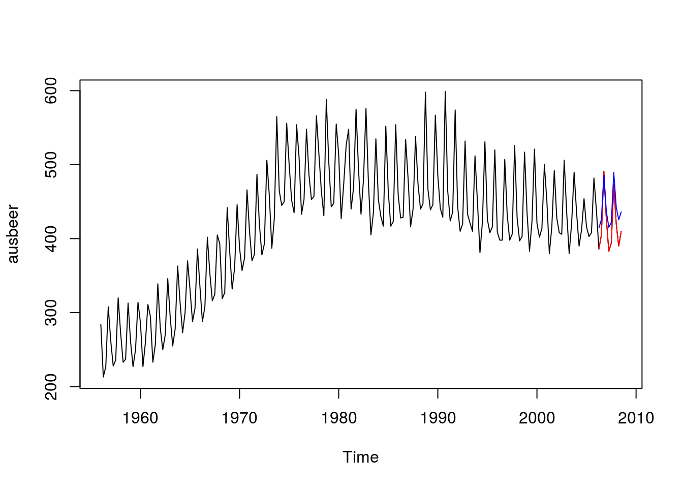

Alternatively, one could reuse the model using

model2 = narx(model, beer_train2)
fcst3 = forecast(model2, h = 10)

plot(fcst3)
lines(fcst2, col="red")

Using exogenous data

Use xreg parameter as exogenous data. This example tries to forecast a random walk. Without xreg, this should be almost impossible:

set.seed(0)

tstamps = seq(as.Date("2000-01-01"), length.out = 110, by='day')
x = xts(runif(length(tstamps)), tstamps)
xreg = 1 - 0.5 * x
yreg = xts(runif(110), tstamps)

colnames(xreg) = colnames(yreg) = "xreg"

# training and testing data
x_train = head(x, 100)
x_test = tail(x, 10)
ind_test = index(x_test)

For simplicity, we use SimpleLM as the learner, which is a simple wrapper for lm. * lm is not compatible with narx as it requires a formula. SimpleLM allows using a linear model without resorting to crafting formulas, similar to what svm from package e1071 does.

Model one, without xreg:

model = narx(x_train, SimpleLM, p = 2)
pred1 = forecast(model, h=10)

Model two, with correlated (good) xreg:

model2 = narx(x_train, SimpleLM, p = 2, xreg = xreg)
pred2 = forecast(model2, xreg=xreg[ind_test])

Model three, with an uncorrelated (bad) xreg:

model3 = narx(x_train, SimpleLM, p = 2, xreg = yreg)
pred3 = forecast(model3, xreg=yreg[ind_test])

The results:

rmse <- function(x,y) sqrt(mean((x-y)^2))

c(Err_without_xreg= rmse(pred1$mean, x_test),
  Err_with_xreg= rmse(pred2$mean, x_test),
  Err_with_bad_xreg= rmse(pred3$mean, x_test))

##  Err_without_xreg     Err_with_xreg Err_with_bad_xreg 
##      2.755231e-01      1.570092e-16      2.985320e-01

The smallest error is obtained from the model with correlated xreg.